Flux tutorial

Load pybhpt.flux

from pybhpt.teuk import TeukolskyMode
from pybhpt.flux import FluxMode
from pybhpt.geo import KerrGeodesic
import numpy as np
import matplotlib.pyplot as plt
import matplotlib as mpl

Solving the inhomogeneous radial Teukolsky equation in Kerr spacetime

The TeukolskyMode class constructs modes of the so-called extended homogeneous solutions to the radial Teukolsky equation for a point-particle source on a bound periodic geodesic,

\[\begin{split}\begin{align} \Psi_s &= \Psi_s^+ \Theta(r-r_p) + \Psi_s^- \Theta(r_p-r), \\ \Psi_s^\pm &= \sum_{jmkn}\Psi^\pm_{sjmkn}(r)S_{sj\gamma_{mkn}}(\theta)e^{im\phi}e^{-i\omega_{mkn}t}, \end{align}\end{split}\]

where we have the mode frequencies \(\omega_{mkn} = m\Omega_\phi + k \Omega_\theta + n \Omega_r\), the discrete spheroidicity \(\gamma_{mkn} = a\omega_{mkn}\), and the extended homogeneous radial solutions

\[ \Psi^\pm_{sjmkn}(r) = Z^{\mathrm{Up/In}}_{sjmkn} R^{\mathrm{Up/In}}_{sjmkn}(r), \]

with Teukolsky amplitudes \(Z^{\mathrm{Up/In}}_{sjmkn}\). The code currently supports spin-weights \(s= 0, \pm 2\), corresponding the scalar perturbations \(\Psi_0 = \Phi\) and curvature perturbations \(\Psi_{2} = \psi_0\), \(\Psi_{-2} = (r-ia\cos\theta)^{4} \psi_4\).

The class is instantiated with the input parameters

• \(s\) : spin-weight of the perturbation

• \(j\) : the spheroidal polar mode number

• \(m\) : the azimuthal mode number

• \(k\) : the polar mode number

• \(n\) : the radial mode number

along with an instance of the KerrGeodesic class that captures the motion of the source.

a, p, e, x = 0.99, 5, 0.6, 0.4
geo = KerrGeodesic(a, p, e, x)

s, j, m, k, n = -2, 12, 3, 1, 2
Psis = TeukolskyMode(s, j, m, k, n, geo)

We solve for the mode solutions and the Teukolsky amplitudes with the solve() method

Psis.solve(geo)

Generating flux contribution from each Teukolsky mode

The time-averaged rate of change of the orbital energy \(\langle \dot{E}\rangle\), angular momentum \(\langle \dot{L}_z\rangle\), and Carter constant \(\langle \dot{Q}\rangle\) can be expressed in terms of the Teukolsky amplitudes \(Z^\mathrm{Up/In}_{sjmkn}\),

\[\begin{split} \begin{align} \langle \dot{\mathcal{J}} \rangle & = \langle \dot{\mathcal{J}} \rangle^\mathrm{inf} + \langle \dot{\mathcal{J}} \rangle^\mathrm{hor}, \\ &= \sum_{jmkn} \langle \dot{\mathcal{J}} \rangle^\mathrm{inf/hor}_{jmkn}, \\ &= \sum_{jmkn} \alpha_{sjmkn}^{(\mathcal{J})\mathrm{inf/hor}}\left| Z^\mathrm{Up/In}_{sjmkn} \right|^2, \end{align}\end{split}\]

where \(\mathcal{J} = (E, L_z, Q)\), \(\alpha_{sjmkn}^{(\mathcal{J})\mathrm{inf}/\mathrm{hor}}\) are known coefficients, and \(s=0, \pm 2\) produce either scalar or gravitational fluxes, respectively.

The FluxMode class takes as input an instances of the Kerr geodesic class and the Teukolsky class for a mode \((s,j,m,k,n)\), and produces the flux contribution for that given mode.

flux = FluxMode(geo, Psis)

Then we can access the horizon fluxes, infinity fluxes, and total fluxes, which are stored in lists with the order of \(\mathcal{J} = (E, L_z, Q)\)

print(flux.horizonfluxes)
print(flux.infinityfluxes)
print(flux.totalfluxes)

[-3.606222842872166e-36, -3.5075219557527026e-35, -1.979059439027494e-34]
[6.753687090778148e-25, 6.56884135710292e-24, 3.7063566971910574e-23]
[6.753687090742086e-25, 6.568841357067845e-24, 3.706356697171267e-23]

Example: Circular Kerr fluxes

As a quick example, we compute the total fluxes for a particle on a circular Kerr geodesic

a, p, e, x = 0.99, 5, 0., 1.
geo = KerrGeodesic(a, p, e, x, nsamples=2**2)

jmax = 18
total_fluxes = np.zeros(3)
horizon_fluxes = np.zeros(3)
infinity_fluxes = np.zeros(3)
total_fluxes_jmodes = np.zeros((jmax - 1, 3))
for j in range(2, jmax+1):
    for m in range(1, j+1):
        Psis = TeukolskyMode(-2, j, m, 0, 0, geo, auto_solve=True)
        flux = FluxMode(geo, Psis)
        total_fluxes += flux.totalfluxes
        total_fluxes_jmodes[j-2] += flux.totalfluxes
        horizon_fluxes += flux.horizonfluxes
        infinity_fluxes += flux.infinityfluxes
total_fluxes *= 2
horizon_fluxes *= 2
infinity_fluxes *= 2
total_fluxes_jmodes *= 2

print("Total fluxes (E, Lz, Q): ", total_fluxes)

Total fluxes (E, Lz, Q):  [0.00122957 0.01496423 0.        ]

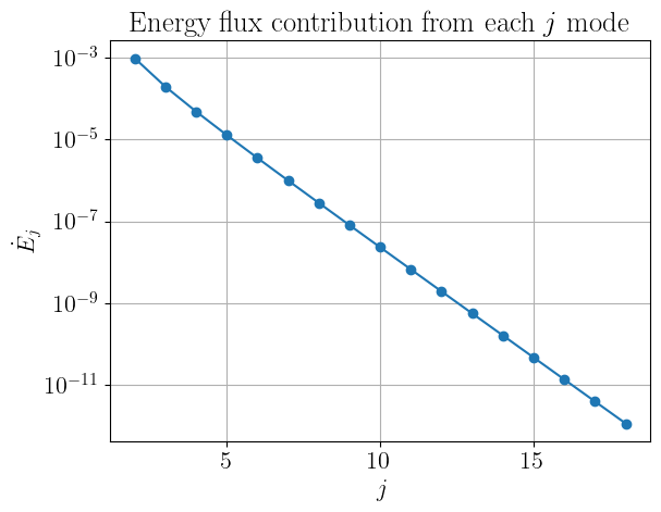
We can also plot the convergence of the mode-sum, which we see falls-off exponentially

mpl.rcParams['text.usetex'] = True
mpl.rcParams['font.family'] = 'serif'
mpl.rcParams['font.size'] = 16

plt.plot(range(2, jmax+1), total_fluxes_jmodes[:, 0], 'o-')
plt.yscale('log')
plt.xlabel('$j$')
plt.ylabel('$\dot{E}_{j}$')
plt.title('Energy flux contribution from each $j$ mode')
plt.grid()
plt.show()