Snapshot waveform tutorial#
Load pybhpt.geo and pybhpt.teuk#
from pybhpt.teuk import TeukolskyMode
from pybhpt.geo import KerrGeodesic
from pybhpt.swsh import SpinWeightedSpheroidalHarmonic
import numpy as np
import matplotlib.pyplot as plt
import matplotlib as mpl
Building a snapshot waveform#
We can build a snapshot waveform produced by a point-particle on a periodic geodesic in Kerr spacetime from the Teukolsky solutions. The snapshot waveform \(h = h_+ - i h_\times\) is related to Teukolsky solutions by \(\psi_4(r\rightarrow\infty) = \frac{1}{2}\ddot{h}\), leading to
First we define a background geodesic
a, p, e, x = 0.99, 5, 0.6, 0.4
geo = KerrGeodesic(a, p, e, x, nsamples = 2**8)
We now build the waveform, starting with computing all amplitudes which contribute to the total power above some threshold tolerance tol
To facilitate the sum over \(k\), and \(n\), we build some functions for computing the amplitudes and checking their relative strength to the sum of the squared amplitudes
def k_mode_sum(j, m, n, geo, modes, n_total_power_sq, total_power_sq, tol = 1e-5, klimit = 10):
    """
    This function computes the sum over $k$-modes for a given set
    of indices $(j, m, n)$ and a geodesic object.
    It iteratively solves the Teukolsky equation for each $k$-mode,
    computes the amplitude, and accumulates the squared power
    until the relative contribution of new modes falls below a
    specified tolerance. The function handles both positive
    and negative $k$ values, skipping unphysical cases.
    Results are appended to the `modes` list
    and the total power is updated.

    Parameters:
    ===========
    - `j, m, n`: Mode indices
    - `geo`: KerrGeodesic object
    - `modes`: List to store mode results
    - `n_total_power_sq`: Accumulated power for this $n$
    - `total_power_sq`: Accumulated total power
    - `tol`: Relative tolerance for convergence (default: 1e-5)
    - `klimit`: Maximum $|k|$ value to sum (default: 10)

    Returns:
    ========
    - Updated `modes` list
    - Updated `n_total_power_sq`
    - Updated `total_power_sq`
    """

    kerror = 1
    kconverge = 0
    k0 = -m
    k = k0
    nk_total_power_sq_prev = 1
    while (k < klimit) and (kconverge < 3):
        if (m == 0) and (n == 0) and (k <= 0):
            k += 1
        else:
            Psis = TeukolskyMode(-2, j, m, k, n, geo)
            Psis.solve(geo)
            amp = -2*Psis.amplitude('Up')/Psis.frequency**2
            if Psis.precision('Up') > 0.01:
                amp = 0

            nk_total_power_sq = np.abs(amp)**2
            n_total_power_sq += nk_total_power_sq
            total_power_sq += nk_total_power_sq

            kerror = np.sqrt(nk_total_power_sq/total_power_sq)
            if (kerror < tol) and (nk_total_power_sq_prev >= nk_total_power_sq):
                kconverge += 1
            else:
                kconverge = 0
            modes.append([j, m, k, n, Psis.frequency, amp])
            k += 1
            nk_total_power_sq_prev = nk_total_power_sq
    # print(n, k-1)

    k = k0 - 1
    kconverge = 0
    nk_total_power_sq_prev = 1
    while (np.abs(k) < klimit) and (kconverge < 3):
        if (m == 0) and (n == 0) and (k <= 0):
            k -= 1
        else:
            Psis = TeukolskyMode(-2, j, m, k, n, geo)
            Psis.solve(geo)
            amp = -2*Psis.amplitude('Up')/Psis.frequency**2
            if Psis.precision('Up') > 0.01:
                amp = 0

            nk_total_power_sq = np.abs(amp)**2
            n_total_power_sq += nk_total_power_sq
            total_power_sq += nk_total_power_sq

            kerror = np.sqrt(nk_total_power_sq/total_power_sq)
            if (kerror < tol) and (nk_total_power_sq_prev >= nk_total_power_sq):
                kconverge += 1
            else:
                kconverge = 0
            modes.append([j, m, k, n, Psis.frequency, amp])
            k -= 1
            nk_total_power_sq_prev = nk_total_power_sq
    # print(n, k+1)

    return modes, n_total_power_sq, total_power_sq
def n_mode_sum(j, m, geo, modes, m_total_power_sq, total_power_sq, tol = 1e-5, nlimit = 50, klimit = 10):
    """
    This function computes the sum over $n$-modes for a given
    $(j, m)$ and geodesic object. For each $n$-mode, it calls
    `k_mode_sum` to perform the $k$-sum, accumulates the squared
    power, and checks for convergence. Both positive and negative
    $n$ values are considered, skipping unphysical cases. Results
    are appended to the `modes` list and the total power is updated.

    Parameters:
    ===========
    - `j, m`: Mode indices
    - `geo`: KerrGeodesic object
    - `modes`: List to store mode results
    - `m_total_power_sq`: Accumulated power for this $m$
    - `total_power_sq`: Accumulated total power
    - `tol`: Relative tolerance for convergence (default: 1e-5)
    - `nlimit`: Maximum $|n|$ value to sum (default: 50)
    - `klimit`: Maximum $|k|$ value to sum (default: 10)

    Returns:
    ========
    - Updated `modes` list
    - Updated `m_total_power_sq`
    - Updated `total_power_sq`
    """
    n0 = 0
    n = n0
    nconverge = 0
    n_total_power_sq_prev = 1
    while (n < nlimit) and (nconverge < 3):
        if (m == 0) and (n < 0):
            n += 1
        else:
            n_total_power_sq = 0.
            modes, n_total_power_sq, total_power_sq = k_mode_sum(j, m, n, geo, modes, n_total_power_sq, total_power_sq, tol=tol, klimit=klimit)
            m_total_power_sq += n_total_power_sq

            nerror = np.sqrt(n_total_power_sq/total_power_sq)
            if (nerror < tol) and (n_total_power_sq_prev >= n_total_power_sq):
                nconverge += 1
            else:
                nconverge = 0
            n += 1
            n_total_power_sq_prev = n_total_power_sq
    # print(n-1)

    n = n0 - 1
    nconverge = 0
    n_total_power_sq_prev = 1
    while (np.abs(n) < nlimit) and (nconverge < 3):
        if (m == 0) and (n < 0):
            n -= 1
        else:
            n_total_power_sq = 0.
            modes, n_total_power_sq, total_power_sq = k_mode_sum(j, m, n, geo, modes, n_total_power_sq, total_power_sq, tol=tol, klimit=klimit)
            m_total_power_sq += n_total_power_sq

            nerror = np.sqrt(n_total_power_sq/total_power_sq)
            if (nerror < tol) and (n_total_power_sq_prev >= n_total_power_sq):
                nconverge += 1
            else:
                nconverge = 0
            n -= 1
            n_total_power_sq_prev = n_total_power_sq
    # print(n+1)

    return modes, m_total_power_sq, total_power_sq
We then specify the tolerance of the amplitude power we want to include in the waveform. To speed up calculations, we set it to 0.01
tol = 1e-2
We then produce all of the relevant modes and store them in a list modes. (This can take several minutes depending on the tolerance set and the nature of the source.)
total_power_sq = 0.
nlimit = 120
klimit = 40

modes = []
jerror = 1
j = 2
jmax = 15
while (j <= jmax) and (jerror > tol):
    m = j
    j_total_power_sq = 0.
    mconvergence = 0
    while m >= 0 and mconvergence < 2:
        print(j, m)

        m_total_power_sq = 0.
        modes, m_total_power_sq, total_power_sq = n_mode_sum(j, m, geo, modes, m_total_power_sq, total_power_sq, tol=tol, nlimit=nlimit, klimit=klimit)
        j_total_power_sq += m_total_power_sq

        merror = np.sqrt(m_total_power_sq/total_power_sq)
        if merror < tol:
            mconvergence += 1
        else:
            mconvergence = 0
        m -= 1
        # print(np.sqrt(m_total_power_sq))
    jerror = np.sqrt(j_total_power_sq/total_power_sq)
    # print(j, jerror, tol, jerror > tol, np.sqrt(total_power_sq))
    j += 1
2 2
2 1
2 0
3 3
3 2
3 1
3 0
4 4
4 3
4 2
4 1
4 0
5 5
5 4
5 3
5 2
5 1
5 0
6 6
6 5
6 4
6 3
6 2
6 1
6 0
7 7
7 6
7 5
7 4
7 3
7 2
7 1
7 0
8 8
8 7
8 6
8 5
8 4
8 3
8 2
8 1
8 0
9 9
9 8
9 7
9 6
9 5
9 4
9 3
9 2
9 1
9 0
10 10
10 9
10 8
10 7
10 6
10 5
10 4
10 3
10 2
10 1
10 0
11 11
11 10
11 9
11 8
11 7
11 6
11 5
11 4
11 3
11 2
11 1
11 0
12 12
12 11
12 10
12 9
12 8
12 7
12 6
12 5
12 4
12 3
12 2
12 1
12 0
13 13
13 12
13 11
13 10
13 9
13 8
13 7
13 6
13 5
13 4
13 3
13 2
13 1
13 0
14 14
14 13
14 12
14 11
14 10
14 9
14 8
14 7
14 6
14 5
14 4
14 3
14 2
14 1
14 0
15 15
15 14
15 13
15 12
15 11
15 10
15 9
15 8
15 7
15 6
15 5
15 4
15 3
15 2
15 1
15 0
We specify the time samples for computing the waveform, along with the polar viewing angles
th = 0.4
phi = 0.2
u_grid = np.linspace(0, 4*2*np.pi/geo.frequencies[0], 800)
We then build the waveform from the selected mode amplitudes
h = 0.j
for mode in modes:
    j, m, k, n, omega, amp = mode
    Slm = SpinWeightedSpheroidalHarmonic(-2, j, m, a*omega)(th)
    h += amp * Slm * np.exp(1j * (m * phi - omega * u_grid))
    Slm = SpinWeightedSpheroidalHarmonic(-2, j, -m, -a*omega)(th)
    h += (-1)**(j + k) * np.conj(amp) * Slm * np.exp(-1j * (m * phi - omega * u_grid))
Plotting the waveform
mpl.rcParams['text.usetex'] = True
mpl.rcParams['font.family'] = 'serif'
mpl.rcParams['font.size'] = 16

plt.plot(u_grid, h.real, label='Re')
plt.plot(u_grid, h.imag, label='Im')
plt.xlabel(r'$u$')
plt.ylabel(r'$d_L \times h$')
plt.legend()
plt.tight_layout()
plt.show()
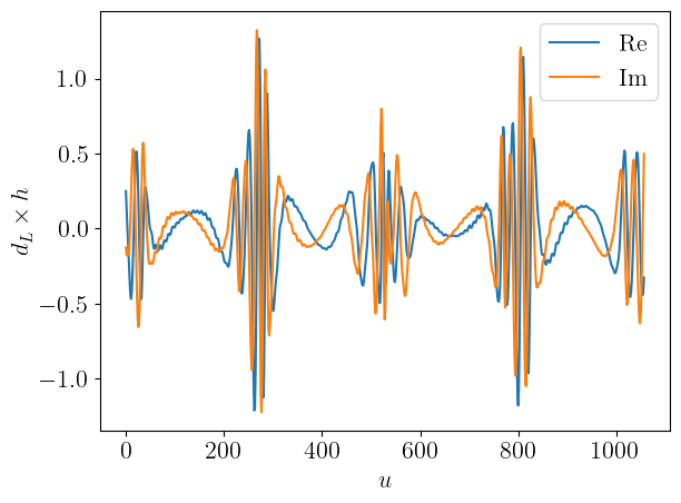
Note that the residual high-frequency oscillations can be mitigated by reducing the value of tol