Radial Teukolsky tutorial

Load pybhpt.radial

from pybhpt.radial import RadialTeukolsky
import numpy as np
import matplotlib.pyplot as plt
import matplotlib as mpl

Solving the homogeneous radial Teukolsky equation in Kerr spacetime

The RadialTeukolsky class solves the homogeneous radial Teukolsky equation

\[\left[\Delta^{-s} \frac{d}{dr} \left(\Delta^{s+1} \frac{d }{dr} \right) + \left(\frac{K^2-2is(r-M)K}{\Delta}+4is\omega r - \lambda_{sjm\omega} \right)\right]R_{sjm\omega} =0\]

given the parameters:

• \(s\) : spin-weight of the perturbation

• \(j\) : the spheroidal polar mode number

• \(m\) : the azimuthal mode number

• \(a\) : the dimensionless Kerr spin parameter

• \(\omega\) : the frequency

where \(\Delta=r^2-2Mr+a^2\), \(K=(r^2+a^2)\omega-ma\), and \(\lambda_{sjm\omega}\) is the spheroidal eigenvalue (separation constant).

In particular we construct the homogeneous solutions \(R^\mathrm{In}_{sjm\omega}\) and \(R^\mathrm{Up}_{sjm\omega}\), which correspond to the asymptotic boundary conditions

\[\begin{split}\begin{align} R^\mathrm{In}_{sjm\omega} (r \rightarrow r_+) &\sim A^\mathrm{trans}_s \Delta^{-s} e^{-i k r_*}, \\ R^\mathrm{In}_{sjm\omega} (r \rightarrow \infty) &\sim A^\mathrm{ref}_s r^{-(2s+1)} e^{i\omega r_*} + A^\mathrm{inc}_s r^{-1} e^{-i\omega r_*}, \\ R^\mathrm{Up}_{sjm\omega} (r \rightarrow r_+) &\sim B^\mathrm{ref}_s \Delta^{-s} e^{-i k r_*} + B^\mathrm{inc}_s e^{i k r_*}, \\ R^\mathrm{Up}_{sjm\omega} (r \rightarrow \infty) &\sim B^\mathrm{trans}_s r^{-(2s+1)} e^{i\omega r_*}, \end{align}\end{split}\]

where \(k = \omega - m \omega_+\), \(\omega_+ = a/(2Mr_+)\), and the tortoise coordinate is given by the differential relation \(dr_{*}/dr = (r^2+a^2)/\Delta\), which can be immediately integrated, leading to

\[r_* = r + \frac{r_+}{\kappa} \ln \frac{r-r_+}{2M} - \frac{r_-}{\kappa} \ln \frac{r-r_-}{2M},\]

where \(\kappa = \sqrt{1 - q^2}\) and \(q = a/M\).

To construct the solutions for some set of radial points \(r\), we first instantiate the class with the Teukolsky parameters \((s, j, m, a, \omega)\) and the points \(r\),

s, j, m, a, omega = -2, 12, 3, 0.99, 2.2
r_hor = 1 + np.sqrt(1 - a**2)
r_grid = np.linspace(r_hor + 2, 100, 3000)
Rt = RadialTeukolsky(s, j, m, a, omega, r_grid)

then we call the solve() method

Rt.solve()

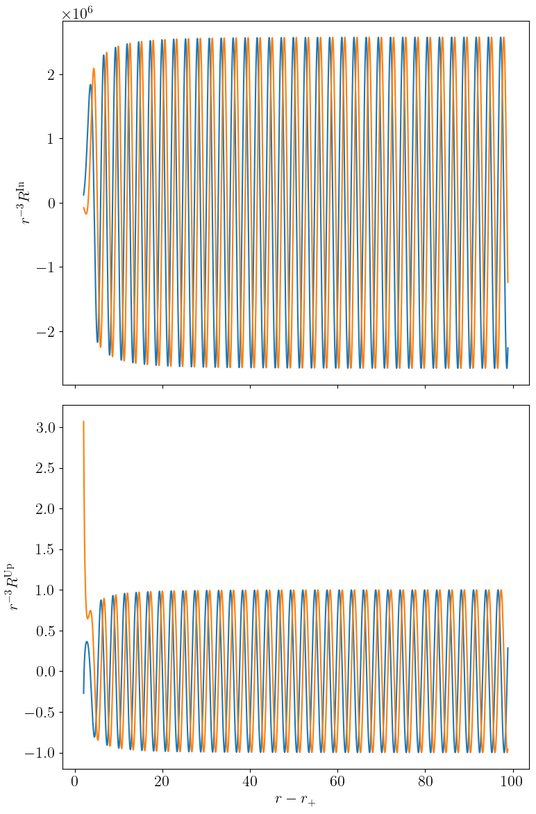
We can then plot the real and imaginary parts of our solutions

mpl.rcParams['text.usetex'] = True
mpl.rcParams['font.family'] = 'serif'
mpl.rcParams['font.size'] = 16

Rin = Rt.radialsolutions('In')
Rup = Rt.radialsolutions('Up')
Delta = r_grid**2 - 2 * r_grid + a**2

fig, axs = plt.subplots(2, 1, figsize=(8, 12), sharex=True)
axs[0].plot(r_grid - r_hor, Rin.real*r_grid**(-3), label='Re')
axs[0].plot(r_grid - r_hor, Rin.imag*r_grid**(-3), label='Im')
axs[0].set_ylabel(r'$r^{-3} R^\mathrm{In}$')

axs[1].plot(r_grid - r_hor, Rup.real*r_grid**(-3), label='Re')
axs[1].plot(r_grid - r_hor, Rup.imag*r_grid**(-3), label='Im')
axs[1].set_ylabel(r'$r^{-3} R^\mathrm{Up}$')
axs[1].set_xlabel(r'$r - r_+$')

plt.tight_layout()
plt.show()