Geodesic tutorial#
Load pybhpt.geo#
from pybhpt.geo import KerrGeodesic
import numpy as np
import matplotlib.pyplot as plt
import matplotlib as mpl
Constructing bound, periodic, timelike geodesics in Kerr#
Bound timelike geodesics are defined in terms of the Keplerian-like parameters:
\(a\) : the dimensionless Kerr spin parameter
\(p\) : the dimensionless semilatus rectum
\(e\) : the orbital eccentricty
\(x\) : cosine of the orbital inclination
The class KerrGeodesics takes in these orbital parameters as input. Additionally, there is the optional parameter nsamples which specifies how many phase-space points are pre-sampled and stored along the geodesic for later computations and classes (e.g., the source integration performed by the TeukolskyMode class).
a, p, e, x, nsamples = (0.9, 8., 0.6, 0.9, 2**9)
geo = KerrGeodesic(a, p, e, x, nsamples)
Accessing orbital constants#
Calling the KerrGeodesic computes the geodesic solutions and all related frequencies and constants of motion. The original orbital parameters are accessible via class properties
(geo.blackholespin, geo.semilatusrectum, geo.eccentricity, geo.inclination) == geo.orbitalparameters
array([ True, True, True, True])
along with the orbital constants: orbital energy \(E\), \(z\)-component of the orbital angular momentum \(L_z\), and Carter constant \(Q\),
(geo.orbitalenergy, geo.orbitalangularmomentum, geo.carterconstant) == geo.orbitalconstants
array([ True, True, True])
the roots of the radial equation,
geo.radialroots
array([20. , 5. , 1.43907677, 0.14948052])
the roots of the polar equation,
geo.polarroots
array([13.13628216, 0.43588989])
the frequencies \(\Upsilon_\alpha\) with respect to Mino time \(\lambda\),
geo.minofrequencies
array([138.1989209 , 2.45185678, 3.24162659, 3.47835419])
and the fundamental frequencies \(\Omega_\alpha\) with respect to coordinate time \(t\),
geo.frequencies, geo.timefrequencies
(array([0.0177415 , 0.02345624, 0.02516918]),
 array([0.0177415 , 0.02345624, 0.02516918]))
Evaluating geodesic solutions#
To evaluate the geodesic solutions \(x^\mu_p(\lambda)=(t_p,r_p,\theta_p,\phi_p)\) at Mino time \(\lambda\), we can simply call the class instance,
la = 10.
geo(la)
array([1.40675551e+03, 5.31917866e+00, 1.33313149e+00, 3.47941508e+01])
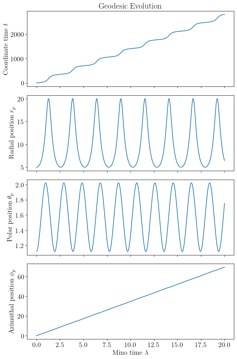
One can also evaluate on a grid of \(\lambda\) values
la_grid = np.linspace(0, 20, 1000)
geo_grid = geo(la_grid)
And then plot the solutions
mpl.rcParams['text.usetex'] = True
mpl.rcParams['font.family'] = 'serif'
mpl.rcParams['font.size'] = 16

fig, axs = plt.subplots(4, 1, figsize=(8, 12), sharex=True)
axs[0].plot(la_grid, geo_grid[0])
axs[0].set_ylabel(r'Coordinate time $t$')
axs[0].set_title(r'Geodesic Evolution')

axs[1].plot(la_grid, geo_grid[1])
axs[1].set_ylabel(r'Radial position $r_p$')

axs[2].plot(la_grid, geo_grid[2])
axs[2].set_ylabel(r'Polar position $\theta_p$')

axs[3].plot(la_grid, geo_grid[3])
axs[3].set_ylabel(r'Azimuthal position $\phi_p$')
axs[3].set_xlabel(r'Mino time $\lambda$')

plt.tight_layout()
plt.show()
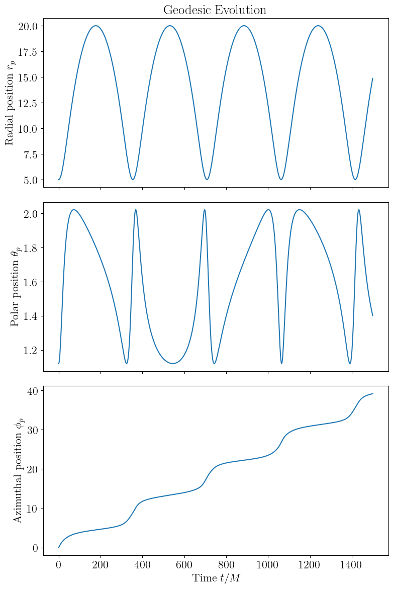
One can also get the evolution as a function of coordinate time by first solving for \(\lambda(t)\)
t_grid = np.linspace(0, 1500, 1000)
la_t_grid = geo.mino_of_t(t_grid)
geo_t_grid = geo(la_t_grid)
mpl.rcParams['text.usetex'] = True
mpl.rcParams['font.family'] = 'serif'
mpl.rcParams['font.size'] = 16

fig, axs = plt.subplots(3, 1, figsize=(8, 12), sharex=True)
axs[0].set_title(r'Geodesic Evolution')
axs[0].plot(t_grid, geo_t_grid[1])
axs[0].set_ylabel(r'Radial position $r_p$')

axs[1].plot(t_grid, geo_t_grid[2])
axs[1].set_ylabel(r'Polar position $\theta_p$')

axs[2].plot(t_grid, geo_t_grid[3])
axs[2].set_ylabel(r'Azimuthal position $\phi_p$')
axs[2].set_xlabel(r'Time $t/M$')

plt.tight_layout()
plt.show()